GPmp Tutorial¶

This tutorial defines a Gaussian process with GPmp, selects covariance parameters, checks predictions, and inspects one-dimensional cross sections of the predictor. It assumes basic knowledge of Gaussian processes. For background on Gaussian-process prediction, see [1, 10, 13]. For parameter selection in GP interpolation, see [9].

Installation and backend selection¶

For an editable installation, first clone the repository, then run pip install -e . from the cloned repository root:

git clone https://github.com/gpmp-dev/gpmp.git
cd gpmp
pip install -e .

GPmp selects its numerical backend at import time. Set GPMP_BACKEND before importing gpmp to choose explicitly:

export GPMP_BACKEND=numpy

or:

export GPMP_BACKEND=torch

If GPMP_BACKEND is not set, GPmp uses PyTorch when available and otherwise falls back to NumPy. Install PyTorch separately when the torch backend is desired.

Basics¶

In kriging, observations are modeled as values of a Gaussian process. The notation \(Z \sim \mathrm{GP}(m,k)\) means that \(Z\) is a Gaussian process with mean function \(m:x\in\mathcal{X}\mapsto\mathrm{E}(Z(x))\) and covariance function \(k:(x,y)\in\mathcal{X}^2\mapsto \mathrm{cov}(Z(x),Z(y))\), with respect to a probability space \((\Omega,\mathcal{B},\mathbb{P}_0)\).

Consider the model \(Z\) defined by:

\[\begin{split}\left\{ \begin{array}{l} Z \sim \mathrm{GP}(m,k), \\ m(\cdot) = \sum_{\ell=1}^q \beta_\ell p_\ell(\cdot), \\ \beta_1,\ldots,\beta_q \in \mathbb{R}, \end{array}\right.\end{split}\]

where the \(\beta_\ell\) are unknown parameters, the \(p_\ell\) are mean basis functions on \(\mathcal X\), and \(k\) is a continuous, strictly positive-definite covariance function.

Parameter selection¶

In GPmp, covariance parameters are stored in a vector covparam. The vector layout depends on the covariance function. The sigma2_rho layout is [log(sigma2), -log(rho_0), ..., -log(rho_{d-1})]. It is used by covariance functions parameterized by a variance and anisotropic lengthscales. The matern sigma2_nu_rho layout is [log(sigma2), log(nu), -log(rho_0), ..., -log(rho_{d-1})].

The choice of selection criterion is part of the GP specification. Petit et al. [9] gives an empirical comparison of parameter-selection criteria in GP interpolation.

Let \(z \in \mathbb{R}^n\) be the vector of observations, \(P \in \mathbb{R}^{n \times q}\) the matrix of mean basis functions evaluated at the observation points, and \(K_\theta \in \mathbb{R}^{n \times n}\) the covariance matrix for covariance parameters \(\theta\).

Maximum likelihood¶

For a parameterized mean \(P\beta\), maximum likelihood minimizes the negative log-likelihood after estimating the mean parameters. With

\[\hat\beta_\theta = \left(P^\top K_\theta^{-1} P\right)^{-1} P^\top K_\theta^{-1} z,\]

the ML criterion is

\[\hat\theta_{\mathrm{ML}} \in \arg\min_\theta \left[ \frac12 \log |K_\theta| + \frac12 (z - P\hat\beta_\theta)^\top K_\theta^{-1}(z - P\hat\beta_\theta) + \frac{n}{2}\log(2\pi) \right].\]

Restricted maximum likelihood¶

Restricted maximum likelihood (REML) uses linear contrasts that eliminate the unknown mean coefficients. Let \(W\in\mathbb{R}^{n\times(n-q)}\) be an orthonormal contrast matrix satisfying

\[W^\top P = 0.\]

In GPmp, \(W\) is built from a complete QR factorization of \(P\), so its columns form an orthonormal basis of the null space of \(P^\top\). The contrast vector \(W^\top z\) has covariance

\[G_\theta = W^\top K_\theta W,\]

and does not depend on \(\beta\). The REML criterion implemented in GPmp is the negative log-likelihood of these contrasts:

\[\hat\theta_{\mathrm{REML}} \in \arg\min_\theta \left[ \frac12 \log |G_\theta| + \frac12 (W^\top z)^\top G_\theta^{-1}(W^\top z) + \frac{n-q}{2}\log(2\pi) \right].\]

This is the restricted likelihood formulation used to select covariance parameters when the mean is a linear predictor [13].

REMAP¶

Restricted maximum a posteriori (REMAP) adds a prior on covariance parameters to the restricted likelihood. If \(\pi(\theta)\) denotes the prior density, GPmp minimizes

\[\hat\theta_{\mathrm{REMAP}} \in \arg\min_\theta \left[ \mathrm{NLRL}(\theta) - \log \pi(\theta) \right],\]

where \(\mathrm{NLRL}\) is the negative log restricted likelihood. The prior can regularize poorly identified covariance parameters. Background on kriging and covariance-parameter conventions is given by Chilès and Delfiner [1], Stein [13]. GPmp provides REMAP functions with priors on \(\log(\sigma^2)\) and on log lengthscales.

Minimal sequence¶

The following code is a complete GPmp sequence on the four-dimensional Hartmann function. It creates observation points, defines mean and covariance functions, selects covariance parameters by REML, and predicts at test points. The observations are treated as noise-free. To use noisy observations or a nugget term, define a covariance function that adds the observation noise on the diagonal. See Noisy observations for a one-dimensional noisy-observation example and Noisy conditional sample paths for heteroscedastic noise in conditional sample paths.

The example pages extend this sequence in several directions: 1D interpolation gives the simplest one-dimensional case, 2D interpolation and Higher-dimensional interpolation show higher-dimensional interpolation, Custom covariance shows how to provide a custom covariance, ML / REML / REMAP parameter selection compares ML, REML, and REMAP, Posterior parameter sampling samples covariance parameters, and Dataloader-based parameter selection uses batched criterion evaluations.

The code below gives the complete setup used by the plots in this tutorial. The mean function returns the matrix of mean basis functions evaluated at x. Here the mean space is the one-dimensional space of constant functions. The covariance parameters are selected by REML. After this call, model.covparam contains the selected covariance parameters and info contains optimization metadata and selection-criterion callables.

Prediction check¶

In dimension four, there is no direct curve to plot. A first check is therefore to compare the posterior mean with reference values at test points.

import gpmp as gp
import gpmp.num as gnp

gnp.set_seed(1234)

dim = 4
box = [[0.0] * dim, [1.0] * dim]

ni = 40
xi = gp.misc.designs.ldrandunif(dim, ni, box)
zi = gp.misc.testfunctions.hartmann4(xi)

nt = 300
xt = gp.misc.designs.ldrandunif(dim, nt, box)
zt = gp.misc.testfunctions.hartmann4(xt)

def constant_mean(x, param):
    return gnp.ones((x.shape[0], 1))

def covariance(x, y, covparam, pairwise=False):
    p = 3
    return gp.kernel.maternp_covariance(x, y, p, covparam, pairwise)

model = gp.Model(constant_mean, covariance)
model, info = gp.kernel.select_parameters_sigma2_rho_with_reml(model, xi, zi, info=True)
zpm, zpv = model.predict(xi, zi, xt)

fig = gp.plot.Figure()
fig.plot(zt, zpm, "ko", markersize=3)
(xmin, xmax), (ymin, ymax) = fig.ax.get_xlim(), fig.ax.get_ylim()
lo = min(xmin, ymin)
hi = max(xmax, ymax)
fig.plot([lo, hi], [lo, hi], "--", linewidth=1)
fig.xylabels("reference values", "posterior mean")
fig.title("Hartmann4: test predictions")
fig.grid()
fig.show()

The resulting plot is:

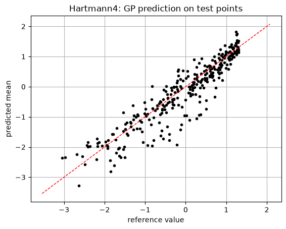
Points close to the dashed reference line indicate accurate prediction. Strong systematic curvature or a large vertical spread would indicate bias or large prediction errors.

Diagnosis output¶

The model-diagnosis tools print the parameter-selection report and prediction-performance metrics:

gp.modeldiagnosis.diag(
    model, "linear_mean_maternp_anisotropic", info, xi, zi
)

zloom, zloov, eloo = model.loo(xi, zi)
gp.modeldiagnosis.perf(
    model,
    xi,
    zi,
    loo=True,
    loo_res=(zloom, zloov, eloo),
    xtzt=(xt, zt),
    zpmzpv=(zpm, zpv),
)

A typical output starts as follows:

[Model diagnosis]
  * Parameter selection
    cvg_reached: True
    optimal_val: True
        n_evals: 19
       final_val: 29.4649
  * Parameters
      sigma2: log variance parameter
       rho_0: log inverse lengthscale, denormalized rho about 0.71
       rho_1: log inverse lengthscale, denormalized rho about 1.23
       rho_2: log inverse lengthscale, denormalized rho about 0.53
       rho_3: log inverse lengthscale, denormalized rho about 0.71

[Prediction performances]
  LOO  (n=40):  Q2 = 0.770, rmse/std(z) = 0.479
  Test (n=300): R2 = 0.599, rmse/std(z) = 0.633

Performance output:

[Prediction performances]
  LOO (n=40)
                     value
          std(z):    0.948
             tss:   35.082
           press:    9.274
       press/tss:    0.264
log10(press/tss):   -0.578
            rmse:    0.482
     rmse/std(z):    0.508
              Q2:    0.736
  Test (n=300)
                   value
        std(z):    1.008
           tss:  303.811
           rss:   44.713
       rss/tss:    0.147
log10(rss/tss):   -0.832
          rmse:    0.386
   rmse/std(z):    0.383
            R2:    0.853

For a block of reference values indexed by \(A\), the total sum of squares is

\[\mathrm{TSS}_A = \sum_{a\in A} (z_a - \bar z_A)^2.\]

For leave-one-out (LOO) prediction, let \(e_i^{\mathrm{LOO}} = z_i - \widehat z_{-i}(x_i)\), where \(\widehat z_{-i}\) is computed without observation \(i\). GPmp reports

\[\mathrm{PRESS} = \sum_i \left(e_i^{\mathrm{LOO}}\right)^2, \qquad Q^2 = 1 - \frac{\mathrm{PRESS}}{\mathrm{TSS}_{\mathrm{obs}}}.\]

For a test set, let \(e_t^{\mathrm{test}} = z_t - \widehat z(x_t)\). GPmp reports

\[\mathrm{RSS} = \sum_t \left(e_t^{\mathrm{test}}\right)^2, \qquad R^2 = 1 - \frac{\mathrm{RSS}}{\mathrm{TSS}_{\mathrm{test}}}.\]

In both blocks, \(\mathrm{RMSE} = \sqrt{\mathrm{SSE}/n}\), with \(\mathrm{SSE}=\mathrm{PRESS}\) for LOO and \(\mathrm{SSE}=\mathrm{RSS}\) for the test set. std(z) is the empirical standard deviation of the reference values in the block. rmse/std(z) is a scale-free error. press/tss and rss/tss are error-to-variance ratios, so smaller values are better.

Check optimizer convergence first: cvg_reached and optimal_val should be true. The parameter block then reports \(\log(\sigma^2)\) and the log inverse lengthscales \(-\log(\rho_j)\). In this Hartmann4 run, the selected lengthscales are of comparable size, which means that the REML criterion does not identify a clearly inactive coordinate. The performance report gives a LOO Q2 and a test-set R2. Values close to one indicate accurate prediction relative to the variance of the observed or test values.

What-if cross sections¶

Prediction cross sections show how predictions change in a local “what-if” analysis. They can be read as a local sweep study around an anchor point. Here the anchor is the observation with the smallest observed value. Starting from this point, one input coordinate is swept through its range while the other coordinates are kept fixed. Each panel shows the posterior mean and Gaussian coverage intervals along that one-dimensional slice. The grey points are the observations projected onto the swept coordinate. They help locate the data but should not be read as values that lie on the conditional slice.

import matplotlib.pyplot as plt

gp.plot.crosssections(model, xi, zi, box, ind_i="min", ind_dim=list(range(dim)))
plt.show()

The resulting plot is:

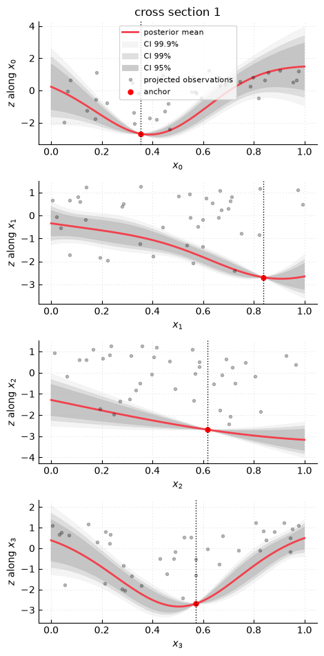
The vertical line marks the coordinate value of the best observed point. These plots should be read as local conditional predictions around that point. They show how the GP predictor changes when one input varies and the others stay fixed. The projected observations show where data are located along each coordinate, but they are not conditional observations on the slice. Wide intervals indicate regions where the model is uncertain along the slice, usually because observations provide little information there.

Leave-one-out diagnostics¶

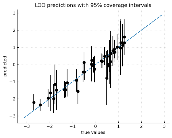
Leave-one-out (LOO) predictions check whether the selected covariance parameters produce predictive intervals consistent with observed errors. In the plot below, each point is an observation predicted from all other observations. The vertical bars show nominal 95% predictive intervals. The same model object is used. No parameter selection is run again.

zloom, zloov, eloo = model.loo(xi, zi)
gp.plot.plot_loo(zi, zloom, zloov)

The resulting plot is:

For selection procedures built through gpmp.kernel, info contains the optimized covariance parameters, optimization history, and criterion callables used by diagnostics and posterior samplers.

REMAP variant¶

The same model can be selected with REMAP by replacing the selection call:

model, info = gp.kernel.select_parameters_sigma2_rho_with_remap_logsigma2_logrho_prior(model, xi, zi, info=True)

For the current default REMAP prior, the prior anchor used for \(\log(\sigma^2)\) and log lengthscales is computed from the standard anisotropic initial guess unless explicit prior anchors are provided.