Higher-dimensional interpolation with Matérn regularity selection
This example is the matern counterpart of Higher-dimensional interpolation. It uses
gp.kernel.matern_covariance and selects nu together with the variance
and lengthscales. The illustration uses the Hartmann4 test function with 80
observation points and 1,000 independent test points in \([0,1]^4\).
What this example does
The script builds a high-dimensional interpolation workflow for Hartmann4:
generate observation and test points in \([0,1]^4\),
build a GP model with a constant mean basis,
select covariance parameters by REML,
predict independent test points,
compute leave-one-out predictions,
inspect one-dimensional prediction cross sections.
The difference is that this example uses a Matérn covariance with continuous
regularity nu and selects nu together with the variance and
lengthscales. The covariance parameter vector is therefore
Mathematical description
The model is
with a constant mean basis. The covariance is anisotropic Matérn with selected
regularity nu:
The scalar correlation function is
Outputs
The diagnosis table reports the selected variance, regularity nu, and
lengthscales.
Note that the call to gp.modeldiagnosis.diag passes
"linear_mean_matern_anisotropic" as model_type.
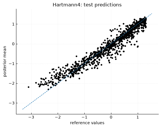
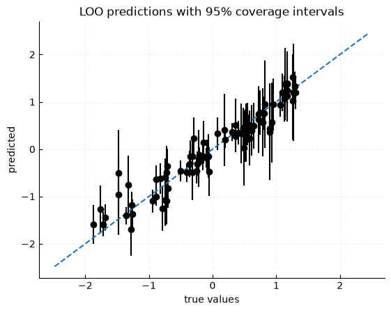
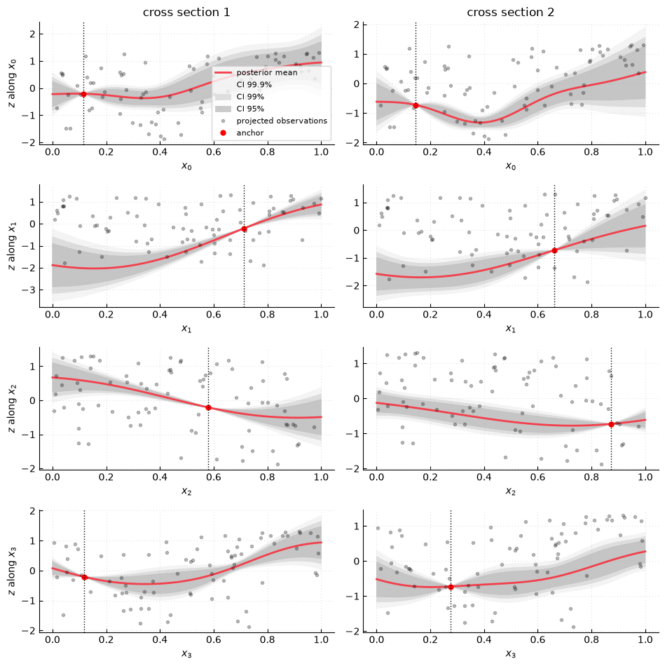
The prediction scatter plot, LOO plot, and cross sections have the same interpretation as in Higher-dimensional interpolation.
Regularity profile
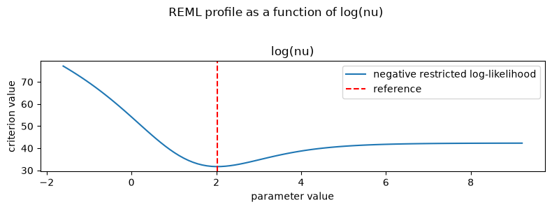
The script also plots a one-dimensional cross section of the REML criterion as
a function of log(nu). This plot checks whether the selected Matérn
regularity is locally identified. A marked minimum means that nearby
regularity values give worse restricted likelihood values. A flat curve means
that several regularities are nearly equivalent for the current observations.
Functions and conventions
gp.kernel.matern_covarianceevaluates the Matérn covariance withnuas a covariance parameter. Its default numerical policy requires no method argument. See Numerical evaluation of the Matérn covariance for the NumPy and Torch evaluation paths.gp.kernel.select_parameters_sigma2_nu_rho_with_remlselects[log(sigma2), log(nu), -log(rho_0), ...]by REML.gpmp.parameter.param_from_covparam_sigma2_nu_rhois the parameter-display helper used by model diagnosis for this covariance convention."linear_mean_matern_anisotropic"tells diagnosis to use thesigma2_nu_rhodisplay convention.gp.modeldiagnosis.plot_selection_criterion_crosssectionsplots the REML criterion profile with respect tolog(nu).
[Model diagnosis]
  * Parameter selection
    cvg_reached: True
    optimal_val: False
        n_evals: 131
           time: 0.2599
    initial_val: 47.0351
      final_val: 31.7001
  * Parameters
      Name:                     Path       Norm             Bounds     Value    Denorm
    sigma2:       covparam->variance        log     [-10.2, 9.803]    -0.186     0.830
        nu:     covparam->regularity        log    [-9.307, 10.69]     2.027     7.594
     rho_0:    covparam->lengthscale    log_inv    [-9.578, 10.42]     0.955     0.385
     rho_1:    covparam->lengthscale    log_inv    [-9.592, 10.41]     0.337     0.714
     rho_2:    covparam->lengthscale    log_inv    [-9.569, 10.43]    0.0851     0.918
     rho_3:    covparam->lengthscale    log_inv    [-9.584, 10.42]     0.760     0.468
  * Data
    count: 80
    -----
              min      max    delta     mean      std delta_over_sigma
     zi:   -1.873    1.304    3.178   0.0204    0.883            3.828
   xi_0:   0.0150    0.992    0.977    0.478    0.292            2.538
   xi_1: 8.323e-3    0.999    0.991    0.494    0.286            1.389
   xi_2: 4.728e-3    0.974    0.969    0.466    0.286            1.055
   xi_3: 4.191e-3    0.988    0.984    0.496    0.284            2.103
[Prediction performances]
  LOO (n=80)
                     value
          std(z):    0.889
             tss:   62.430
           press:    5.410
       press/tss:   0.0867
log10(press/tss):   -1.062
            rmse:    0.260
     rmse/std(z):    0.293
              Q2:    0.913
  Test (n=1000)
                   value
        std(z):    1.021
           tss:  1.041e3
           rss:   74.549
       rss/tss:   0.0716
log10(rss/tss):   -1.145
          rmse:    0.273
   rmse/std(z):    0.267
            R2:    0.928
Script: examples/gpmp_example31_nd_matern.py
  1"""Higher-dimensional interpolation with Matérn regularity selection.
  2
  3This example mirrors ``gpmp_example04_nd.py`` but uses
  4``gp.kernel.matern_covariance`` instead of the fixed-regularity
  5``gp.kernel.maternp_covariance``. The covariance parameter vector is
  6
  7    [log(sigma2), log(nu), -log(rho_0), ..., -log(rho_{d-1})],
  8
  9so the Matérn regularity ``nu`` is selected together with the variance and
 10lengthscales.
 11
 12----
 13Author: Emmanuel Vazquez <emmanuel.vazquez@centralesupelec.fr>
 14Copyright (c) 2022-2026, CentraleSupelec
 15License: GPLv3 (see LICENSE)
 16"""
 17
 18import gpmp as gp
 19import gpmp.num as gnp
 20
 21
 22def choose_test_case(problem):
 23    if problem == 1:
 24        problem_name = "Hartmann4"
 25        f = gp.misc.testfunctions.hartmann4
 26        dim = 4
 27        box = [[0.0] * 4, [1.0] * 4]
 28        ni = 80
 29        xi = gp.misc.designs.ldrandunif(dim, ni, box)
 30        nt = 1000
 31        xt = gp.misc.designs.ldrandunif(dim, nt, box)
 32
 33    elif problem == 2:
 34        problem_name = "Hartmann6"
 35        f = gp.misc.testfunctions.hartmann6
 36        dim = 6
 37        box = [[0.0] * 6, [1.0] * 6]
 38        ni = 300
 39        xi = gp.misc.designs.ldrandunif(dim, ni, box)
 40        nt = 1000
 41        xt = gp.misc.designs.ldrandunif(dim, nt, box)
 42
 43    elif problem == 3:
 44        problem_name = "Borehole"
 45        f = gp.misc.testfunctions.borehole
 46        dim = 8
 47        box = [
 48            [0.05, 100.0, 63070.0, 990.0, 63.1, 700.0, 1120.0, 9855.0],
 49            [0.15, 50000.0, 115600.0, 1110.0, 116.0, 820.0, 1680.0, 12045.0],
 50        ]
 51        ni = 30
 52        xi = gp.misc.designs.maximinldlhs(dim, ni, box)
 53        nt = 1000
 54        xt = gp.misc.designs.ldrandunif(dim, nt, box)
 55
 56    elif problem == 4:
 57        problem_name = "detpep8d"
 58        f = gp.misc.testfunctions.detpep8d
 59        dim = 8
 60        box = [[0.0] * 8, [1.0] * 8]
 61        ni = 60
 62        xi = gp.misc.designs.maximinldlhs(dim, ni, box)
 63        nt = 1000
 64        xt = gp.misc.designs.ldrandunif(dim, nt, box)
 65
 66    elif problem == 5:
 67        problem_name = "Ishigami"
 68        f = gp.misc.testfunctions.ishigami
 69        dim = 3
 70        box = [[-gnp.pi] * 3, [gnp.pi] * 3]
 71        ni = 50
 72        xi = gp.misc.designs.ldrandunif(dim, ni, box)
 73        nt = 1000
 74        xt = gp.misc.designs.ldrandunif(dim, nt, box)
 75
 76    return problem_name, f, dim, box, ni, xi, nt, xt
 77
 78
 79def constant_mean(x, param):
 80    return gnp.ones((x.shape[0], 1))
 81
 82
 83def visualize_predictions(problem_name, zt, zpm):
 84    fig = gp.plot.Figure()
 85    fig.plot(zt, zpm, "ko", markersize=3)
 86    (xmin, xmax), (ymin, ymax) = fig.ax.get_xlim(), fig.ax.get_ylim()
 87    xmin = min(xmin, ymin)
 88    xmax = max(xmax, ymax)
 89    fig.plot([xmin, xmax], [xmin, xmax], "--", linewidth=1)
 90    fig.xylabels("reference values", "posterior mean")
 91    fig.title(f"{problem_name}: test predictions")
 92    fig.grid()
 93    fig.show()
 94
 95
 96def main():
 97    problem = 1
 98    problem_name, f, dim, box, ni, xi, nt, xt = choose_test_case(problem)
 99
100    zi = f(xi)
101    zt = f(xt)
102
103    model = gp.Model(constant_mean, gp.kernel.matern_covariance)
104    model, info = gp.kernel.select_parameters_sigma2_nu_rho_with_reml(
105        model, xi, zi, info=True
106    )
107    gp.modeldiagnosis.diag(
108        model,
109        "linear_mean_matern_anisotropic",
110        info,
111        xi,
112        zi,
113    )
114    gp.modeldiagnosis.plot_selection_criterion_crosssections(
115        info=info,
116        ind=[1],
117        param_names=["log(sigma2)", "log(nu)"]
118        + [f"-log(rho_{j})" for j in range(dim)],
119        param_box=[[gnp.log(0.2)], [gnp.log(10000.0)]],
120        n_points=100,
121        criterion_name="negative restricted log-likelihood",
122        criterion_name_full="REML profile as a function of log(nu)",
123    )
124
125    (zpm, zpv) = model.predict(xi, zi, xt)
126
127    visualize_predictions(problem_name, zt, zpm)
128
129    zloom, zloov, eloo = model.loo(xi, zi)
130    gp.plot.plot_loo(zi, zloom, zloov)
131
132    gp.plot.crosssections(
133        model, xi, zi, box, ind_i=[0, 1], ind_dim=list(range(dim))
134    )
135
136    gp.modeldiagnosis.perf(
137        model,
138        xi,
139        zi,
140        loo=True,
141        loo_res=(zloom, zloov, eloo),
142        xtzt=(xt, zt),
143        zpmzpv=(zpm, zpv),
144    )
145
146
147if __name__ == "__main__":
148    main()