Plotting Matern covariances¶

This example plots Matern covariance kernels with half-integer smoothness parameters. It is the smallest example in the documentation and shows the shape of the kernels used by the interpolation and regression examples.

What this example does¶

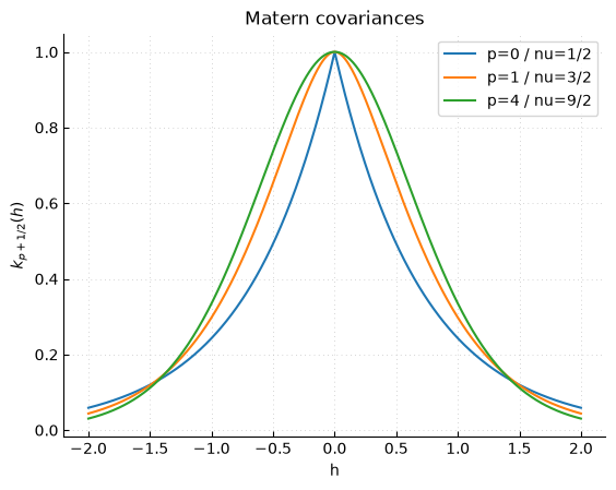
The script builds a one-dimensional grid of scaled distances h and evaluates gp.kernel.maternp_kernel(p, abs(h)) for several integer values of p. For half-integer Matern kernels, nu = p + 1/2. Increasing p produces smoother sample paths and a covariance function that is flatter near the origin.

Mathematical object¶

The function maternp_kernel returns the correlation part of a stationary Matern covariance. For \(\nu = p + 1/2\), GPmp evaluates

\[c_p(h) = \exp(-2\sqrt{\nu}\,h) \frac{\Gamma(p+1)}{\Gamma(2p+1)} \sum_{j=0}^{p} \frac{(p+j)!}{j!(p-j)!} \left(4\sqrt{\nu}\,h\right)^{p-j}.\]

The full anisotropic covariance used in later examples has the form

\[k_\theta(x, x') = \sigma^2 c_p\left( \left\| \left((x_1-x'_1)/\rho_1,\ldots,(x_d-x'_d)/\rho_d\right) \right\|_2 \right).\]

Outputs¶

All curves are normalized to one at h = 0. The curve with p = 0 is the exponential kernel and decays sharply away from the origin. Larger p values produce stronger local smoothness and a slower initial decay. No observations or parameter selection are involved.

API points¶

gp.kernel.maternp_kernel evaluates the correlation kernel as a function of scaled distance.
gp.plot.Figure is a lightweight Matplotlib wrapper used throughout the examples.
For full covariance matrices with variance and lengthscales, use gp.kernel.maternp_covariance instead.

""" Plot the Matern nu = p + 1/2 kernel/covariance functions

Author: Emmanuel Vazquez <emmanuel.vazquez@centralesupelec.fr>
Copyright (c) 2022, CentraleSupelec
License: GPLv3 (see LICENSE)
"""
import gpmp.num as gnp
import gpmp as gp

def main():
    h = gnp.linspace(-2.0, 2.0, 500)

    fig = gp.plot.Figure()

    for p in [0, 1, 4]:
        r = gp.kernel.maternp_kernel(p, gnp.abs(h))
        fig.plot(h, r, label='p={} / nu={}/2'.format(p, 2*p+1))

    fig.title('Matern covariances')
    fig.xlabel('h')
    fig.ylabel('$k_{p+1/2}(h)$')
    fig.legend()
    fig.show(grid=True)


if __name__ == '__main__':
    main()