Higher-dimensional interpolation
This example applies anisotropic Matern GP interpolation to a test function in dimension greater than two. Since direct contour plots are no longer available, the preview uses prediction scatter plots, leave-one-out (LOO) diagnostics, and one-dimensional cross sections.
What this example does
The script chooses a benchmark function, evaluates it at observation points, selects covariance parameters with REMAP, predicts independent test points, and computes LOO predictions. LOO prediction removes one observation at a time, predicts it from all other observations, and compares the prediction with the removed value.
Mathematical object
The model remains
and zi stores realized values \(z_i\). The input dimension is too large
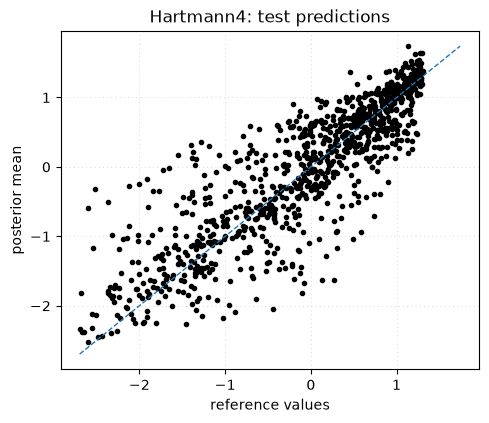
for a direct contour plot. The first diagnostic therefore compares realized
reference values \(z_t\) with the posterior mean
\(\mathbb{E}[Z_t\mid Z_i=z_i]\) on independent test points.
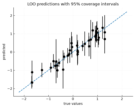
For the LOO diagnostic, each observation is predicted after removing it from the conditioning set:
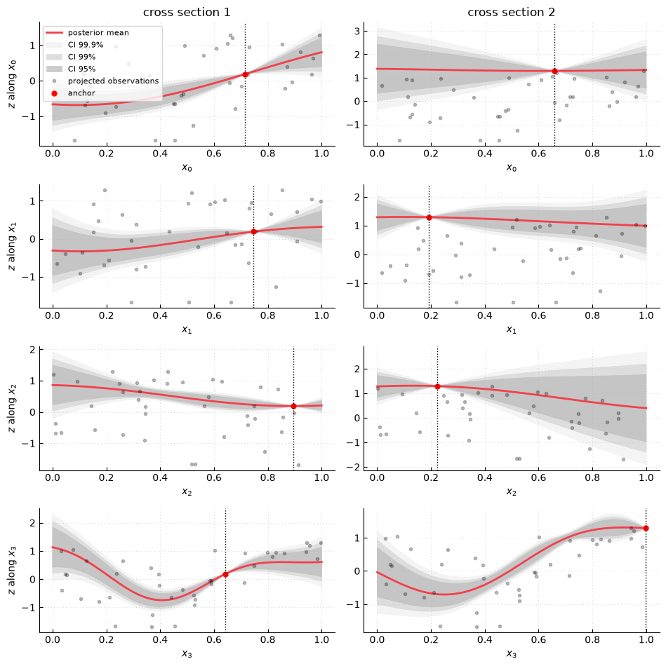
The cross-section plots fix all coordinates except one and display \(x_j \mapsto \mathbb{E}[Z(x)\mid Z_i=z_i]\) and its pointwise uncertainty.
Outputs
The first figure compares GP posterior means with reference values on independent test points. Points close to the diagonal indicate small test errors.
The second figure compares LOO predictions with observed values. Vertical bars show nominal predictive intervals. Large deviations from the diagonal or many observations outside the intervals indicate poorly selected covariance parameters, missing structure, or predictive intervals that are too narrow.
The last figure shows prediction cross sections. Each panel fixes all coordinates except one and plots the posterior mean and intervals along that coordinate. Black points are projected observations. The red point is the observation used as the cross-section anchor.
API points
model.loo(xi, zi)returns LOO means, variances, and errors.gp.plot.plot_looprovides a compact diagnostic for high-dimensional problems where spatial plots are impossible.gp.plot.crosssectionsplots one-dimensional slices through selected observation points.REMAP parameter selection can be used when pure likelihood criteria produce poorly identified lengthscales.
Script: examples/gpmp_example04_nd.py
  1"""Prediction of some classical test functions in dimension > 2
  2
  3An anisotropic Matern covariance function is used for the Gaussian
  4Process (GP) prior. The parameters of this covariance function
  5(variance and ranges) are estimated using the Restricted Maximum
  6A Posteriori (ReMAP).
  7
  8The mean function of the GP prior is assumed to be constant and
  9unknown.
 10
 11The function is sampled on a space-filling Latin Hypercube design, and
 12the data is assumed to be noiseless.
 13
 14----
 15Author: Emmanuel Vazquez <emmanuel.vazquez@centralesupelec.fr>
 16Copyright (c) 2022-2026, CentraleSupelec
 17License: GPLv3 (see LICENSE)
 18"""
 19import gpmp.num as gnp
 20import gpmp as gp
 21import matplotlib.pyplot as plt
 22
 23
 24def choose_test_case(problem):
 25    if problem == 1:
 26        problem_name = "Hartmann4"
 27        f = gp.misc.testfunctions.hartmann4
 28        dim = 4
 29        box = [[0.0] * 4, [1.0] * 4]
 30        ni = 40
 31        xi = gp.misc.designs.ldrandunif(dim, ni, box)
 32        nt = 1000
 33        xt = gp.misc.designs.ldrandunif(dim, nt, box)
 34
 35    elif problem == 2:
 36        problem_name = "Hartmann6"
 37        f = gp.misc.testfunctions.hartmann6
 38        dim = 6
 39        box = [[0.0] * 6, [1.0] * 6]
 40        ni = 200
 41        xi = gp.misc.designs.ldrandunif(dim, ni, box)
 42        nt = 1000
 43        xt = gp.misc.designs.ldrandunif(dim, nt, box)
 44
 45    elif problem == 3:
 46        problem_name = "Borehole"
 47        f = gp.misc.testfunctions.borehole
 48        dim = 8
 49        box = [
 50            [0.05, 100.0, 63070.0, 990.0, 63.1, 700.0, 1120.0, 9855.0],
 51            [0.15, 50000.0, 115600.0, 1110.0, 116.0, 820.0, 1680.0, 12045.0],
 52        ]
 53        ni = 30
 54        xi = gp.misc.designs.maximinldlhs(dim, ni, box)
 55        nt = 1000
 56        xt = gp.misc.designs.ldrandunif(dim, nt, box)
 57
 58    elif problem == 4:
 59        problem_name = "detpep8d"
 60        f = gp.misc.testfunctions.detpep8d
 61        dim = 8
 62        box = [[0.0] * 8, [1.0] * 8]
 63        ni = 60
 64        xi = gp.misc.designs.maximinldlhs(dim, ni, box)
 65        nt = 1000
 66        xt = gp.misc.designs.ldrandunif(dim, nt, box)
 67
 68    elif problem == 5:
 69        problem_name = "Ishigami"
 70        f = gp.misc.testfunctions.ishigami
 71        dim = 3
 72        box = [[-gnp.pi] * 3, [gnp.pi] * 3]
 73        ni = 80
 74        xi = gp.misc.designs.ldrandunif(dim, ni, box)
 75        nt = 1000
 76        xt = gp.misc.designs.ldrandunif(dim, nt, box)
 77
 78    return problem_name, f, dim, box, ni, xi, nt, xt
 79
 80
 81def constant_mean(x, param):
 82    return gnp.ones((x.shape[0], 1))
 83
 84
 85def kernel(x, y, covparam, pairwise=False):
 86    p = 10
 87    return gp.kernel.maternp_covariance(x, y, p, covparam, pairwise)
 88
 89
 90def visualize_predictions(problem_name, zt, zpm):
 91    plt.figure()
 92    plt.plot(zt, zpm, "ko")
 93    (xmin, xmax), (ymin, ymax) = plt.xlim(), plt.ylim()
 94    xmin = min(xmin, ymin)
 95    xmax = max(xmax, ymax)
 96    plt.plot([xmin, xmax], [xmin, xmax], "--")
 97    plt.title(problem_name)
 98    plt.show()
 99
100
101def main():
102    problem = 5
103    problem_name, f, dim, box, ni, xi, nt, xt = choose_test_case(problem)
104
105    zi = f(xi)
106    zt = f(xt)
107
108    model = gp.Model(constant_mean, kernel)
109    model, info = gp.kernel.select_parameters_with_remap(model, xi, zi, info=True)
110    gp.modeldiagnosis.diag(model, info, xi, zi)
111
112    (zpm, zpv) = model.predict(xi, zi, xt)
113
114    visualize_predictions(problem_name, zt, zpm)
115
116    zloom, zloov, eloo = model.loo(xi, zi)
117    gp.plot.plot_loo(zi, zloom, zloov)
118
119    gp.plot.crosssections(
120        model, xi, zi, box, ind_i=[0, 1], ind_dim=list(range(dim))
121    )
122
123    gp.modeldiagnosis.perf(
124        model,
125        xi,
126        zi,
127        loo=True,
128        loo_res=(zloom, zloov, eloo),
129        xtzt=(xt, zt),
130        zpmzpv=(zpm, zpv),
131    )
132
133
134if __name__ == "__main__":
135    main()