1D interpolation
This example builds a one-dimensional noise-free Gaussian process model and
selects covariance parameters by restricted maximum likelihood (REML). It is the
recommended first complete example because it shows the basic GPmp sequence:
construct a model, select covparam, predict, and plot the result.
What this example does
The script creates observation points xi and observations zi from a
known reference function. It defines a constant-mean GP with an anisotropic
Matérn covariance and calls
gp.kernel.select_parameters_sigma2_rho_with_reml. The selected covariance
parameters are stored in model.covparam and are then used by
model.predict on a dense grid xt.
The method name encodes the parameter layout and the criterion. sigma2_rho
means [log(sigma2), -log(rho_0), ..., -log(rho_{d-1})]. with_reml means
that the optimizer minimizes the negative restricted log-likelihood. The method
also supplies the matching anisotropic initial guess when covparam0 is not
provided.
Mathematical description
The noise-free observation model is
where the trend coefficients \(\beta\) are unknown. In this example,
constant_mean gives a constant trend basis, so \(p(x)=1\).
After selecting \(\theta\), model.predict(xi, zi, xt) computes the
universal, or intrinsic, kriging predictor [1, 13].
Let \(P_i\) be the trend matrix at the observation points, \(P_t\) the
trend matrix at prediction points, \(K_{ii}\) the observation covariance
matrix, \(K_{it}\) the covariance block between observations and
prediction points, and \(K_{tt}\) the covariance block at prediction
points. The kriging weights \(\Lambda\) and Lagrange multipliers
\(M\) solve
The posterior mean and covariance are then
and
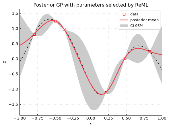
The plotted uncertainty envelope is built from the diagonal of the conditional covariance.
Outputs
The displayed quantities are the reference function, the observations, the posterior mean, and the posterior uncertainty envelope. Because the observations are treated as noise-free, the posterior mean interpolates the observed values. The uncertainty is small near observations and larger away from them.
Functions used
Use
gpmp.core.Modelorgp.Modelto assemble a mean function and a covariance function.Use
select_parameters_sigma2_rho_with_remlwhen REML is used with the[log(sigma2), -log(rho_0), ...]covariance-parameter convention.Use
model.predict(xi, zi, xt)to compute posterior mean and variance at prediction points.
Script: examples/gpmp_example02_1d_interpolation.py
  1"""
  2One-dimensional GP interpolation with REML parameter selection.
  3
  4Author: Emmanuel Vazquez <emmanuel.vazquez@centralesupelec.fr>
  5Copyright (c) 2022-2026, CentraleSupelec
  6License: GPLv3 (see LICENSE)
  7"""
  8
  9import gpmp.num as gnp
 10import gpmp as gp
 11import gpmp.plot as gpplot
 12
 13
 14def generate_data():
 15    """
 16    Data generation.
 17
 18    Returns
 19    -------
 20    tuple
 21        (xt, zt): target data
 22        (xi, zi): input dataset
 23    """
 24    dim = 1
 25    nt = 200
 26    box = [[-1], [1]]
 27    xt = gp.misc.designs.regulargrid(dim, nt, box)
 28    zt = gp.misc.testfunctions.twobumps(xt)
 29
 30    ni = 6  # FIXME improve stability for ni > 50
 31    xi = gp.misc.designs.ldrandunif(dim, ni, box)
 32    zi = gp.misc.testfunctions.twobumps(xi)
 33
 34    return xt, zt, xi, zi
 35
 36
 37def constant_mean(x, param):
 38    return gnp.ones((x.shape[0], 1))
 39
 40
 41def kernel(x, y, covparam, pairwise=False):
 42    p = 3
 43    return gp.kernel.maternp_covariance(x, y, p, covparam, pairwise)
 44
 45
 46def visualize_results(xt, zt, xi, zi, zpm, zpv):
 47    """
 48    Visualize the results using gp.plot (a matplotlib wrapper).
 49
 50    Parameters
 51    ----------
 52    xt : numpy.ndarray
 53        Target x values
 54    zt : numpy.ndarray
 55        Target z values
 56    xi : numpy.ndarray
 57        Input x values
 58    zi : numpy.ndarray
 59        Input z values
 60    zpm : numpy.ndarray
 61        Posterior mean
 62    zpv : numpy.ndarray
 63        Posterior variance
 64    """
 65    fig = gpplot.Figure(isinteractive=True)
 66    fig.plot(xt, zt, "k", linewidth=1, linestyle=(0, (5, 5)))
 67    fig.plotdata(xi, zi)
 68    fig.plotgp(xt, zpm, zpv, colorscheme="simple")
 69    fig.xylabels("$x$", "$z$")
 70    fig.title("Posterior GP with parameters selected by REML")
 71    fig.show(grid=True, xlim=[-1.0, 1.0], legend=True, legend_fontsize=9)
 72
 73
 74def main():
 75    xt, zt, xi, zi = generate_data()
 76
 77    model = gp.Model(constant_mean, kernel)
 78
 79    # Parameter selection by REML.
 80    # The sigma2_rho part states the covparam layout used by this Matérn
 81    # model: [log(sigma2), -log(rho_0), ...].
 82    model, info = gp.kernel.select_parameters_sigma2_rho_with_reml(
 83        model, xi, zi, info=True
 84    )
 85    gp.modeldiagnosis.diag(
 86        model, "linear_mean_maternp_anisotropic", info, xi, zi
 87    )
 88
 89    # Prediction
 90    zpm, zpv = model.predict(xi, zi, xt)
 91
 92    # Visualization
 93    print("\nVisualization")
 94    print("-------------")
 95    plot_likelihood_cross_sections = True
 96    plot_likelihood_2d_profile = False
 97    if plot_likelihood_cross_sections:
 98        gp.modeldiagnosis.plot_selection_criterion_crosssections(
 99            info=info, delta=0.8, param_names=["sigma^2 (log)", "rho (log)"]
100        )
101    if plot_likelihood_2d_profile:
102        gp.modeldiagnosis.plot_selection_criterion_sigma_rho(model, info)
103
104    visualize_results(xt, zt, xi, zi, zpm, zpv)
105
106
107if __name__ == "__main__":
108    main()