ML / REML / REMAP parameter selection
This example compares the main covariance-parameter selection criteria used in GPmp: maximum likelihood (ML), restricted maximum likelihood (REML), and restricted maximum a posteriori (REMAP). The scripts use the same one-dimensional interpolation setup so that only the selection criterion changes.
What this example does
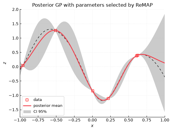
The rendered preview uses REMAP, selects covariance parameters, and plots the
posterior prediction. The full scripts below expose the corresponding REMAP,
REML, and ML procedures. All three procedures optimize a scalar criterion over
covparam but differ in how they handle mean parameters and prior
regularization.
Mathematical criteria
Let \(h_i\) denote the matrix of mean basis functions evaluated at the observation points, and let \(k_{ii}(\theta)\) be the covariance matrix. For a linear mean \(m_\beta(x)=h(x)^\top\beta\), ML profiles out \(\beta\) and minimizes, up to constants independent of \(\theta\),
REML adds the determinant term associated with the estimated mean coefficients:
REMAP adds prior regularization on covariance parameters:
How to interpret the comparison
ML optimizes the likelihood after estimating mean parameters. REML accounts for the degrees of freedom used by the mean and is often preferable when the mean is unknown. REMAP adds prior terms to the restricted likelihood. This may stabilize poorly identified variance or lengthscale parameters. Different criteria can lead to different posterior uncertainty, even when the posterior mean looks similar.
API points
select_parameters_with_remlis the standard restricted-likelihood helper.select_parameters_with_remapand the more explicit REMAP variants add prior regularization.The returned
infoobject records the selectedcovparam, optimization status, objective history, and criterion callables.
REMAP
Script: examples/gpmp_example20_1d_interpolation_variation_remap.py
 1"""
 2Plot and optimize the restricted negative log-likelihood
 3
 4Author: Emmanuel Vazquez <emmanuel.vazquez@centralesupelec.fr>
 5Copyright (c) 2022-2026, CentraleSupelec
 6License: GPLv3 (see LICENSE)
 7"""
 8
 9import gpmp.num as gnp
10import gpmp as gp
11import matplotlib.pyplot as plt
12
13
14def generate_data():
15    """
16    Data generation.
17
18    Returns
19    -------
20    tuple
21        (xt, zt): target data
22        (xi, zi): input dataset
23    """
24    dim = 1
25    nt = 200
26    box = [[-1], [1]]
27    xt = gp.misc.designs.regulargrid(dim, nt, box)
28    zt = gp.misc.testfunctions.twobumps(xt)
29
30    ni = 6
31    xi = gp.misc.designs.ldrandunif(dim, ni, box)
32    zi = gp.misc.testfunctions.twobumps(xi)
33
34    return xt, zt, xi, zi
35
36
37def constant_mean(x, param):
38    return gnp.ones((x.shape[0], 1))
39
40
41def kernel(x, y, covparam, pairwise=False):
42    p = 3
43    return gp.kernel.maternp_covariance(x, y, p, covparam, pairwise)
44
45
46def visualize_results(xt, zt, xi, zi, zpm, zpv):
47    """
48    Visualize the results using gp.plot.plotutils (a matplotlib wrapper).
49
50    Parameters
51    ----------
52    xt : numpy.ndarray
53        Target x values
54    zt : numpy.ndarray
55        Target z values
56    xi : numpy.ndarray
57        Input x values
58    zi : numpy.ndarray
59        Input z values
60    zpm : numpy.ndarray
61        Posterior mean
62    zpv : numpy.ndarray
63        Posterior variance
64    """
65    fig = gp.plot.Figure(isinteractive=True)
66    fig.plot(xt, zt, "k", linewidth=1, linestyle=(0, (5, 5)))
67    fig.plotdata(xi, zi)
68    fig.plotgp(xt, zpm, zpv, colorscheme="simple")
69    fig.xylabels("$x$", "$z$")
70    fig.title("Posterior GP with parameters selected by ReMAP")
71    fig.show(grid=True, xlim=[-1.0, 1.0], legend=True, legend_fontsize=9)
72
73
74def main():
75    xt, zt, xi, zi = generate_data()
76
77    model = gp.core.Model(constant_mean, kernel)
78
79    # Automatic selection of parameters using REMAP
80    model, info = gp.kernel.select_parameters_with_remap(model, xi, zi, info=True)
81    gp.modeldiagnosis.diag(model, info, xi, zi)
82
83    # Prediction
84    zpm, zpv = model.predict(xi, zi, xt)
85
86    # Visualization
87    print("\nVisualization")
88    print("-------------")
89    plot_likelihood = True
90    if plot_likelihood:
91        gp.modeldiagnosis.plot_selection_criterion_sigma_rho(
92            model, info, criterion_name="restricted maximum a posteriori"
93        )
94
95    visualize_results(xt, zt, xi, zi, zpm, zpv)
96
97
98if __name__ == "__main__":
99    main()
REML
Script: examples/gpmp_example21_1d_interpolation_variation_reml.py
  1"""
  2Plot and optimize the restricted negative log-likelihood
  3
  4Author: Emmanuel Vazquez <emmanuel.vazquez@centralesupelec.fr>
  5Copyright (c) 2022-2026, CentraleSupelec
  6License: GPLv3 (see LICENSE)
  7"""
  8
  9import gpmp.num as gnp
 10import gpmp as gp
 11import matplotlib.pyplot as plt
 12
 13
 14def generate_data():
 15    """
 16    Data generation.
 17
 18    Returns
 19    -------
 20    tuple
 21        (xt, zt): target data
 22        (xi, zi): input dataset
 23    """
 24    dim = 1
 25    nt = 200
 26    box = [[-1], [1]]
 27    xt = gp.misc.designs.regulargrid(dim, nt, box)
 28    zt = gp.misc.testfunctions.twobumps(xt)
 29
 30    ni = 8
 31    xi = gp.misc.designs.ldrandunif(dim, ni, box)
 32    zi = gp.misc.testfunctions.twobumps(xi)
 33
 34    return xt, zt, xi, zi
 35
 36
 37def constant_mean(x, param):
 38    return gnp.ones((x.shape[0], 1))
 39
 40
 41def kernel(x, y, covparam, pairwise=False):
 42    p = 3
 43    return gp.kernel.maternp_covariance(x, y, p, covparam, pairwise)
 44
 45
 46def visualize_results(xt, zt, xi, zi, zpm, zpv):
 47    """
 48    Visualize the results using gp.plot.plotutils (a matplotlib wrapper).
 49
 50    Parameters
 51    ----------
 52    xt : numpy.ndarray
 53        Target x values
 54    zt : numpy.ndarray
 55        Target z values
 56    xi : numpy.ndarray
 57        Input x values
 58    zi : numpy.ndarray
 59        Input z values
 60    zpm : numpy.ndarray
 61        Posterior mean
 62    zpv : numpy.ndarray
 63        Posterior variance
 64    """
 65    fig = gp.plot.Figure(isinteractive=True)
 66    fig.plot(xt, zt, "k", linewidth=1, linestyle=(0, (5, 5)))
 67    fig.plotdata(xi, zi)
 68    fig.plotgp(xt, zpm, zpv, colorscheme="simple")
 69    fig.xylabels("$x$", "$z$")
 70    fig.title("Posterior GP with parameters selected by ReML")
 71    fig.show(xlim=[-1.0, 1.0])
 72
 73
 74def main():
 75    xt, zt, xi, zi = generate_data()
 76
 77    meanparam0 = None
 78    covparam0 = None
 79    model = gp.core.Model(constant_mean, kernel, meanparam0, covparam0)
 80
 81    # Parameter initial guess
 82    covparam0 = gp.kernel.anisotropic_parameters_initial_guess(model, xi, zi)
 83
 84    # selection criterion
 85    selection_criterion = gp.kernel.negative_log_restricted_likelihood
 86    nlrl, nlrl_pregrad, nlrl_nograd, dnlrl = gp.kernel.make_selection_criterion_with_gradient(
 87        model, selection_criterion, xi, zi
 88    )
 89
 90    # optimize parameters
 91    covparam_reml, info = gp.kernel.autoselect_parameters(
 92        covparam0, nlrl_pregrad, dnlrl, silent=False, info=True
 93    )
 94
 95    model.covparam = gnp.asarray(covparam_reml)
 96    info["covparam0"] = covparam0
 97    info["covparam"] = covparam_reml
 98    info["selection_criterion"] = nlrl
 99
100    gp.modeldiagnosis.diag(model, info, xi, zi)
101
102    # Prediction
103    zpm, zpv = model.predict(xi, zi, xt)
104
105    # Visualization
106    print("\nVisualization")
107    print("-------------")
108    visualize_results(xt, zt, xi, zi, zpm, zpv)
109
110    zloom, zloov, eloo = model.loo(xi, zi)
111    gp.plot.plot_loo(zi, zloom, zloov)
112
113
114if __name__ == "__main__":
115    main()
ML
Script: examples/gpmp_example22_1d_interpolation_variation_ml.py
  1"""
  2Plot and optimize the restricted negative log-likelihood
  3
  4Author: Emmanuel Vazquez <emmanuel.vazquez@centralesupelec.fr>
  5Copyright (c) 2022-2026, CentraleSupelec
  6License: GPLv3 (see LICENSE)
  7"""
  8
  9import gpmp.num as gnp
 10import gpmp as gp
 11import matplotlib.pyplot as plt
 12
 13
 14def generate_data():
 15    """
 16    Data generation.
 17
 18    Returns
 19    -------
 20    tuple
 21        (xt, zt): target data
 22        (xi, zi): input dataset
 23    """
 24    c = 1.0
 25    dim = 1
 26    nt = 200
 27    box = [[-1], [1]]
 28    xt = gp.misc.designs.regulargrid(dim, nt, box)
 29    zt = gp.misc.testfunctions.twobumps(xt) + c
 30
 31    ni = 8
 32    xi = gp.misc.designs.ldrandunif(dim, ni, box)
 33    zi = gp.misc.testfunctions.twobumps(xi) + c
 34
 35    return xt, zt, xi, zi
 36
 37
 38def constant_mean(x, param):
 39    return param * gnp.ones((x.shape[0], 1))
 40
 41
 42def kernel(x, y, covparam, pairwise=False):
 43    p = 3
 44    return gp.kernel.maternp_covariance(x, y, p, covparam, pairwise)
 45
 46
 47def visualize_results(xt, zt, xi, zi, zpm, zpv):
 48    """
 49    Visualize the results using gp.plot.plotutils (a matplotlib wrapper).
 50
 51    Parameters
 52    ----------
 53    xt : numpy.ndarray
 54        Target x values
 55    zt : numpy.ndarray
 56        Target z values
 57    xi : numpy.ndarray
 58        Input x values
 59    zi : numpy.ndarray
 60        Input z values
 61    zpm : numpy.ndarray
 62        Posterior mean
 63    zpv : numpy.ndarray
 64        Posterior variance
 65    """
 66    fig = gp.plot.Figure(isinteractive=True)
 67    fig.plot(xt, zt, "k", linewidth=1, linestyle=(0, (5, 5)))
 68    fig.plotdata(xi, zi)
 69    fig.plotgp(xt, zpm, zpv, colorscheme="bw")
 70    fig.xylabels("$x$", "$z$")
 71    fig.title("Posterior GP with parameters selected by ML")
 72    fig.show(xlim=[-1.0, 1.0])
 73
 74
 75def main():
 76    xt, zt, xi, zi = generate_data()
 77
 78    meanparam0 = None
 79    covparam0 = None
 80    model = gp.core.Model(
 81        constant_mean, kernel, meanparam0, covparam0, meantype="parameterized"
 82    )
 83
 84    # Parameter initial guess
 85    (
 86        meanparam0,
 87        covparam0,
 88    ) = gp.kernel.anisotropic_parameters_initial_guess_constant_mean(model, xi, zi)
 89
 90    param0 = gnp.concatenate((meanparam0, covparam0))
 91
 92    # selection criterion
 93    nll, nll_pregrad, nll_nograd, dnll = gp.kernel.make_selection_criterion_with_gradient(
 94        model,
 95        gp.kernel.negative_log_likelihood,
 96        xi,
 97        zi,
 98        parameterized_mean=True,
 99        meanparam_len=1,
100    )
101
102    param_ml, info = gp.kernel.autoselect_parameters(
103        param0, nll_pregrad, dnll, silent=False, info=True
104    )
105
106    model.meanparam = gnp.asarray(param_ml[0])
107    model.covparam = gnp.asarray(param_ml[1:])
108
109    info["covparam0"] = param0[1:]
110    info["covparam"] = param_ml[1:]
111    info["selection_criterion"] = nll
112
113    gp.modeldiagnosis.diag(model, info, xi, zi)
114
115    # Prediction
116    zpm, zpv = model.predict(xi, zi, xt)
117
118    # Visualization
119    print("\nVisualization")
120    print("-------------")
121    visualize_results(xt, zt, xi, zi, zpm, zpv)
122
123    zloom, zloov, eloo = model.loo(xi, zi)
124    gp.plot.plot_loo(zi, zloom, zloov)
125
126    return model
127
128
129if __name__ == "__main__":
130    model = main()