Posterior parameter sampling
This example demonstrates REMAP-based parameter selection followed by posterior
sampling of GP covariance parameters. It is intended for cases where point
estimates of covparam are not enough and uncertainty over covariance
parameters should be explored explicitly.
What this example does
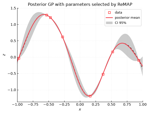
The rendered preview performs REMAP parameter selection and plots the posterior prediction. The full script continues by sampling the posterior distribution of covariance parameters with MCMC methods. For documentation build time, the rendered preview stops before the expensive sampling loop.
Mathematical target
The samplers work on the covariance-parameter vector \(\theta=\mathrm{covparam}\). With the REMAP criterion used in the script, the posterior target is represented through the negative log density
where \(C\) does not depend on \(\theta\). Equivalently,
The MCMC output explores uncertainty over \(\theta\); it is separate from the conditional uncertainty of \(Z_t=Z(x_t)\) for a fixed \(\theta\).
How to interpret the sampling procedure
REMAP provides a regularized starting point and prior definition. Posterior sampling then explores nearby and competing covariance-parameter values according to the selection criterion interpreted as a negative log density. The resulting chains or particles can be used to assess whether the selected covariance parameters are well identified.
API points
select_parameters_with_remap_gaussian_logsigma2_and_logrho_priorselects a regularized covariance vector and defines criterion callables ininfo.Posterior samplers in
gpmp.mcmcuseinfo.selection_criterion_nogradas a negative log-density when possible.Use sampling diagnostics before interpreting posterior parameter samples.
Script: examples/gpmp_example23_1d_interpolation_posterior_sampling.py
  1"""
  2Demonstrates ReMAP-based GP parameter selection, posterior sampling,
  3and visualization of a 1D Gaussian process model.
  4
  5Author: Emmanuel Vazquez <emmanuel.vazquez@centralesupelec.fr>
  6Copyright (c) 2022-2026, CentraleSupelec
  7License: GPLv3 (see LICENSE)
  8"""
  9
 10import gpmp.num as gnp
 11import gpmp as gp
 12from gpmp.mcmc.param_posterior import (
 13    sample_from_selection_criterion_mh,
 14    sample_from_selection_criterion_nuts,
 15)
 16import matplotlib.pyplot as plt
 17from matplotlib import interactive
 18
 19
 20def generate_data():
 21    """
 22    Data generation.
 23
 24    Returns
 25    -------
 26    tuple
 27        (xt, zt): target data
 28        (xi, zi): input dataset
 29    """
 30    dim = 1
 31    nt = 200
 32    box = [[-1], [1]]
 33    xt = gp.misc.designs.regulargrid(dim, nt, box)
 34    zt = gp.misc.testfunctions.twobumps(xt)
 35
 36    ni = 8
 37    xi = gp.misc.designs.ldrandunif(dim, ni, box)
 38    zi = gp.misc.testfunctions.twobumps(xi)
 39
 40    return xt, zt, xi, zi
 41
 42
 43def constant_mean(x, param):
 44    return gnp.ones((x.shape[0], 1))
 45
 46
 47def kernel(x, y, covparam, pairwise=False):
 48    p = 3
 49    return gp.kernel.maternp_covariance(x, y, p, covparam, pairwise)
 50
 51
 52def visualize_results(xt, zt, xi, zi, zpm, zpv):
 53    """
 54    Visualize the results using gp.plot.plotutils (a matplotlib wrapper).
 55
 56    Parameters
 57    ----------
 58    xt : numpy.ndarray
 59        Target x values
 60    zt : numpy.ndarray
 61        Target z values
 62    xi : numpy.ndarray
 63        Input x values
 64    zi : numpy.ndarray
 65        Input z values
 66    zpm : numpy.ndarray
 67        Posterior mean
 68    zpv : numpy.ndarray
 69        Posterior variance
 70    """
 71    fig = gp.plot.Figure(isinteractive=True)
 72    fig.plot(xt, zt, "k", linewidth=1, linestyle=(0, (5, 5)))
 73    fig.plotdata(xi, zi)
 74    fig.plotgp(xt, zpm, zpv, colorscheme="simple")
 75    fig.xylabels("$x$", "$z$")
 76    fig.title("Posterior GP with parameters selected by ReMAP")
 77    fig.show(grid=True, xlim=[-1.0, 1.0], legend=True, legend_fontsize=9)
 78
 79
 80def main():
 81    xt, zt, xi, zi = generate_data()
 82
 83    model = gp.core.Model(constant_mean, kernel)
 84
 85    # Automatic selection of parameters using ReMAP
 86    model, info = (
 87        gp.kernel.select_parameters_with_remap_gaussian_logsigma2_and_logrho_prior(
 88            model, xi, zi, info=True
 89        )
 90    )
 91    gp.modeldiagnosis.diag(model, info, xi, zi)
 92
 93    # Prediction
 94    zpm, zpv = model.predict(xi, zi, xt)
 95
 96    sampler = "nuts"  # "mh" or "nuts"
 97    n_chains = 4
 98    nuts_init_box = None
 99    if hasattr(info, "bounds") and info.bounds is not None:
100        nuts_init_box = [
101            [b[0] for b in info.bounds],
102            [b[1] for b in info.bounds],
103        ]
104
105    if sampler == "mh":
106        samples, _sampler_state = sample_from_selection_criterion_mh(
107            info,
108            n_steps_total=10_000,
109            burnin_period=5_000,
110            n_chains=n_chains,
111            show_progress=True,
112        )
113    elif sampler == "nuts":
114        samples, _sampler_state = sample_from_selection_criterion_nuts(
115            info,
116            num_samples=500,
117            num_warmup=1_000,
118            n_chains=n_chains,
119            init_box=nuts_init_box,
120            progress=True,
121        )
122    else:
123        raise ValueError("Unknown sampler. Use 'mh' or 'nuts'.")
124
125    # Visualization
126    print("\nVisualization")
127    print("-------------")
128    interactive(True)
129    plot_likelihood_cross_sections = True
130    plot_likelihood_2d_profile = True
131    if plot_likelihood_cross_sections:
132        gp.modeldiagnosis.plot_selection_criterion_crosssections(
133            info=info, delta=0.6, param_names=["log(sigma^2)", "log(1/rho)"]
134        )
135    if plot_likelihood_2d_profile:
136        gp.modeldiagnosis.plot_selection_criterion_sigma_rho(
137            model, info, criterion_name="log posterior"
138        )
139
140    plt.scatter(
141        gnp.log10(gnp.exp(samples[0, :, 0] / 2)),
142        gnp.log10(gnp.exp(-samples[0, :, 1])),
143        alpha=0.2,
144    )
145
146    visualize_results(xt, zt, xi, zi, zpm, zpv)
147
148
149if __name__ == "__main__":
150    main()