2D interpolation
This example builds an anisotropic Matern GP on a two-dimensional test function. It illustrates the same modeling sequence as the 1D interpolation example, but with a two-dimensional input space and contour plots for spatial diagnostics.
What this example does
The script selects a two-dimensional test function, draws observation points,
constructs a GP model, and selects covariance parameters with a REMAP criterion.
The covariance vector follows the GPmp convention
[log(sigma2), -log(rho_0), -log(rho_1)]. The selected model is evaluated on
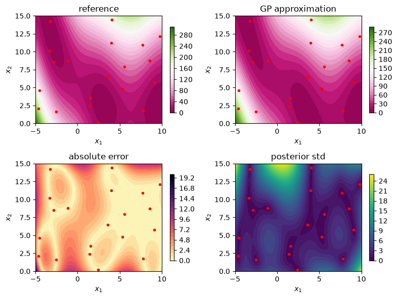
a regular grid to compare the reference function and the GP approximation.
Mathematical object
The model is the same noise-free conditional GP as in the 1D interpolation example, but with two-dimensional points \(x=(x_1,x_2)\). The anisotropic Matern kernel uses the scaled distance
The two lengthscales control smoothing along the two coordinate axes. Small \(\rho_j\) allows faster variation along coordinate \(j\); large \(\rho_j\) makes the posterior vary more slowly along that coordinate.
Outputs
The four panels contain the reference function, GP posterior mean, absolute prediction error, and posterior standard deviation. Red dots mark observation points. The error and posterior standard deviation panels should be read together: a well-calibrated model should assign larger uncertainty in regions with sparse observations or difficult extrapolation.
API points
gp.misc.designs.ldrandunifcreates a space-filling observation design.gp.kernel.select_parameters_with_remapselects covariance parameters with the default REMAP criterion.model.predictreturns posterior means and variances at the grid points.Convert backend arrays with
gnp.to_npbefore sending them to Matplotlib functions that expect NumPy arrays.
Script: examples/gpmp_example03_2d.py
  1"""
  2Gaussian processes in 2D
  3
  4An anisotropic Matern covariance function is used for the Gaussian
  5Process (GP) prior. The parameters of this covariance function
  6(variance and ranges) are estimated using the Restricted Maximum
  7A Posteriori (ReMAP) method.
  8
  9The mean function of the GP prior is assumed to be constant and
 10unknown.
 11
 12The function is sampled on a space-filling Latin Hypercube design, and
 13the data is assumed to be noiseless.
 14
 15----
 16Author: Emmanuel Vazquez <emmanuel.vazquez@centralesupelec.fr>
 17Copyright (c) 2022-2026, CentraleSupelec
 18License: GPLv3 (see LICENSE)
 19----
 20This example is based on the file stk_example_kb03.m from the STK at
 21https://github.com/stk-kriging/stk/
 22by Julien Bect and Emmanuel Vazquez, released under the GPLv3 license.
 23
 24Original copyright notice:
 25
 26   Copyright (c) 2015, 2016, 2018 CentraleSupelec
 27   Copyright (c) 2011-2014 SUPELEC
 28----
 29"""
 30
 31import numpy as np
 32import gpmp.num as gnp
 33import gpmp as gp
 34import matplotlib.pyplot as plt
 35
 36
 37# Test function selection
 38def select_test_function(case_num):
 39    if case_num == 1:
 40        f = gp.misc.testfunctions.braninhoo
 41        dim = 2
 42        box = [[-5, 0], [10, 15]]
 43        ni = 20
 44    elif case_num == 2:
 45        f = gp.misc.testfunctions.wave
 46        dim = 2
 47        box = [[-1, -1], [1, 1]]
 48        ni = 40
 49    return f, dim, box, ni
 50
 51
 52def create_model():
 53    def constant_mean(x, param):
 54        return gnp.ones((x.shape[0], 1))
 55
 56    def kernel(x, y, covparam, pairwise=False):
 57        p = 6
 58        return gp.kernel.maternp_covariance(x, y, p, covparam, pairwise)
 59
 60    return gp.Model(constant_mean, kernel)
 61
 62
 63def main():
 64    case_num = 1
 65    f, dim, box, ni = select_test_function(case_num)
 66
 67    # Compute the function on a 80 x 80 regular grid
 68    nt = [80, 80]
 69    xt = gp.misc.designs.regulargrid(dim, nt, box)
 70    zt = f(xt)
 71
 72    design_type = "ld"
 73    if design_type == "lhs":
 74        xi = gp.misc.designs.maximinlhs(dim, ni, box)
 75    elif design_type == "ld":
 76        xi = gp.misc.designs.ldrandunif(dim, ni, box)
 77    zi = f(xi)
 78
 79    model = create_model()
 80
 81    # Parameter selection
 82    model, info = gp.kernel.select_parameters_with_remap(model, xi, zi, info=True)
 83    gp.modeldiagnosis.diag(model, info, xi, zi)
 84
 85    # Prediction
 86    (zpm, zpv) = model.predict(xi, zi, xt)
 87
 88    # Visualization
 89    contour_lines = 30
 90    xt_np = gnp.to_np(xt)
 91    xi_np = gnp.to_np(xi)
 92    zt_np = gnp.to_np(zt).reshape(nt)
 93    zpm_np = gnp.to_np(zpm).reshape(nt)
 94    zsd_np = np.sqrt(np.maximum(gnp.to_np(zpv).reshape(nt), 0.0))
 95
 96    fig, axes = plt.subplots(nrows=2, ncols=2)
 97    data = [zt_np, zpm_np, np.abs(zpm_np - zt_np), zsd_np]
 98    titles = [
 99        "function to be approximated",
100        f"approximation from {ni} points",
101        "true approx error",
102        "posterior std",
103    ]
104    cmaps = ["PiYG", "PiYG", "magma_r", "viridis"]
105
106    for ax, z, title, cmap in zip(axes.flat, data, titles, cmaps):
107        cs = ax.contourf(
108            xt_np[:, 0].reshape(nt),
109            xt_np[:, 1].reshape(nt),
110            z,
111            levels=contour_lines,
112            cmap=cmap,
113        )
114        ax.plot(xi_np[:, 0], xi_np[:, 1], "ro", label="data")
115        ax.set_title(title)
116        ax.set_xlabel("$x_1$")
117        ax.set_ylabel("$x_2$")
118        ax.legend()
119        fig.colorbar(cs, ax=ax, shrink=0.9)
120
121    plt.show()
122
123    # Predictions vs truth
124    plt.figure()
125    plt.plot(zt, zpm, "ko")
126    (xmin, xmax), (ymin, ymax) = plt.xlim(), plt.ylim()
127    xmin = min(xmin, ymin)
128    xmax = max(xmax, ymax)
129    plt.plot([xmin, xmax], [xmin, xmax], "--")
130    plt.xlabel("true values")
131    plt.ylabel("predictions")
132    plt.show()
133
134    # LOO predictions
135    zloom, zloov, eloo = model.loo(xi, zi)
136    gp.plot.plot_loo(zi, zloom, zloov)
137
138    gp.plot.crosssections(model, xi, zi, box, ind_i=[0, 10], ind_dim=[0, 1])
139
140
141if __name__ == "__main__":
142    main()