Getting started
The first example builds a gpmp-contrib model from observation points. It
uses the four-dimensional Hartmann function, as in the core gpmp tutorial.
The first displayed output is a predicted-versus-reference check on test
points.
The example runs these operations:
choose a
ComputerExperiment.choose observation points and evaluate the experiment.
create a Matérn model container.
select covariance parameters.
predict at test points.
inspect diagnostics and stored model state.
Model construction
import gpmp as gp
import gpmp.num as gnp
import gpmpcontrib as gpc

gnp.set_seed(1234)

problem = gpc.test_problems.hartmann4
box = problem.input_box

xi = gp.misc.designs.ldrandunif(problem.input_dim, 40, box)
zi = problem(xi)

xt = gp.misc.designs.ldrandunif(problem.input_dim, 300, box)
zt = problem(xt)

model = gpc.Model_ConstantMean_Maternp_REML(
    "hartmann4",
    output_dim=problem.output_dim,
    mean_specification={"type": "constant"},
    covariance_specification={"p": 3},
)

model.select_params(xi, zi)
zpm, zpv = model.predict(xi, zi, xt)
print(zpm.shape, zpv.shape)

model.run_diagnosis(xi, zi)
model.run_perf(xi, zi, xtzt=(xt, zt), zpmzpv=(zpm, zpv))

param = model[0].get_param()
covparam = model[0]["model"].covparam
info = model[0]["info"]
The call to gnp.set_seed makes the design reproducible. The prediction
arrays are NumPy arrays by default because ModelContainer.predict uses
convert_out=True.
Objects and stored state
problemThe
ComputerExperiment. It stores the input box, input dimension, output dimension, and callable function. Built-in test problems are available ingpmpcontrib.test_problems.xiandziObservation points and observed values. Here
xihas shape(40, 4). For this scalar-output problem,zihas one column.xtandztTest points and reference values. They are used only to check predictions. They are not used during parameter selection.
modelA
ModelContainersubclass. It stores onegpmp.core.Modelper output. Here there is only one output, so output0stores the Hartmann4 GP model.select_paramsBuilds the REML criterion, chooses an optimizer start, runs SciPy, and stores the selected covariance parameters.
predictComputes posterior means and variances at the test points
xt.
Expected output
The exact optimizer values depend on the random design and on the active numerical backend. The prediction shapes are fixed:
(300, 1) (300, 1)
This line is produced by print(zpm.shape, zpv.shape) in the code above.
The diagnosis output has one block per output:
~ Model [0]
[Model diagnosis]
  * Parameter selection
    cvg_reached: True
    optimal_val: True
    ...
  * Parameters
    ...
  * Data
    count: 40
This block is produced by model.run_diagnosis(xi, zi).
cvg_reached is the SciPy optimizer success flag. optimal_val means that
the final criterion value is finite and usable. The parameter table prints raw
coordinates and denormalized values. For Matérn lengthscales, the raw vector
stores -log(rho) while the denormalized column reports rho.
Prediction check
The code below produces the prediction check from zt and zpm:
import gpmp as gp

zt_ = zt.reshape(-1)
zpm_ = zpm.reshape(-1)
zmin = min(float(zt_.min()), float(zpm_.min()))
zmax = max(float(zt_.max()), float(zpm_.max()))

fig = gp.plot.Figure()
fig.plot(zt_, zpm_, "ko", markersize=3)
fig.plot([zmin, zmax], [zmin, zmax], "k--", linewidth=1)
fig.xylabels("reference value", "posterior mean")
fig.grid()
fig.show()
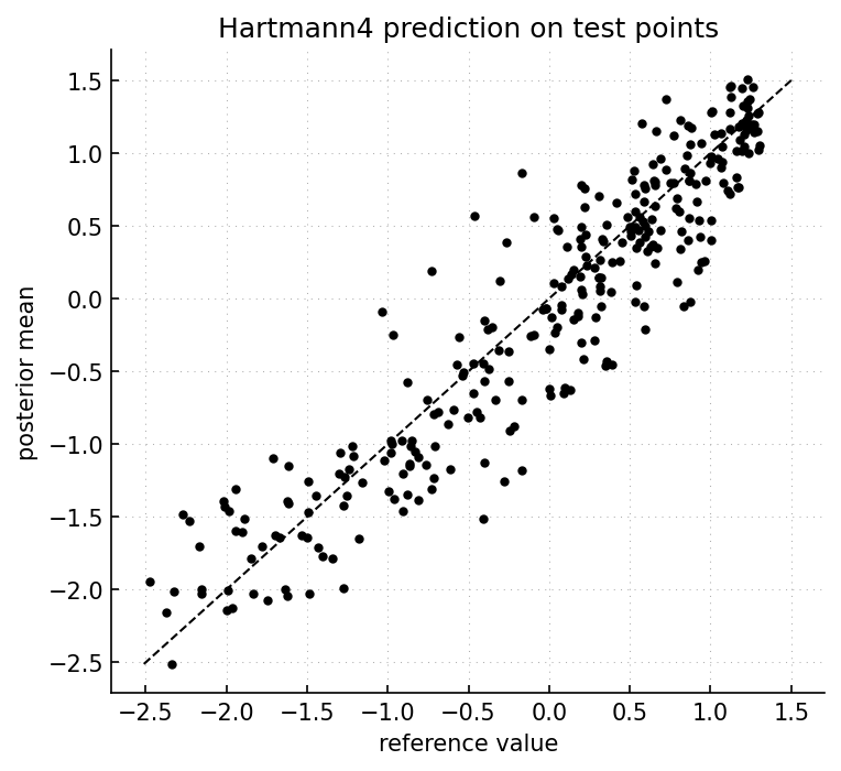
Posterior mean against reference values on 300 test points. Points close to the diagonal indicate accurate prediction. Curvature or a large vertical spread would indicate bias or large prediction errors.
Inspecting the selected model
The selected model state is stored per output:
entry = model[0]
gp_model = entry["model"]

covparam = gp_model.covparam
meanparam = gp_model.meanparam
param = entry.get_param()
info = entry["info"]
covparam is the raw covariance vector passed to gpmp.kernel:
[log(sigma2), -log(rho_0), -log(rho_1), -log(rho_2), -log(rho_3)]
param is the readable Param object. It gives names, paths,
normalization rules, bounds, raw values, and denormalized values. Use it when
inspecting parameters or passing a named optimizer start back to
select_params.
info is the optimizer report. It also stores
selection_criterion_nograd, which is the criterion callable to use for
plots, diagnosis, and posterior parameter sampling when gradients are not
needed.
Checking prediction performance
run_perf prints leave-one-out and test-set summaries:
model.run_perf(xi, zi, xtzt=(xt, zt), zpmzpv=(zpm, zpv))
zloom, zloov, eloo = model.loo(xi, zi)
The displayed block is produced by
model.run_perf(xi, zi, xtzt=(xt, zt), zpmzpv=(zpm, zpv)). For the seeded
Hartmann4 run above, the output is:
~ Model [0]
[Prediction performances]
  LOO (n=40)
                     value
          std(z):    1.047
             tss:   43.829
           press:   11.259
       press/tss:    0.257
log10(press/tss):   -0.590
            rmse:    0.531
     rmse/std(z):    0.507
              Q2:    0.743
  Test (n=300)
                   value
        std(z):    0.989
           tss:  293.704
           rss:   41.061
       rss/tss:    0.140
log10(rss/tss):   -0.854
          rmse:    0.370
   rmse/std(z):    0.374
            R2:    0.860
For each output, the displayed quantities are defined as follows. For reference values \(z_i\),
For leave-one-out prediction, let \(e_i^{\mathrm{LOO}} = z_i - \widehat z_{-i}(x_i)\), where \(\widehat z_{-i}\) is computed without observation \(i\). Then
For a test set, let \(e_i^{\mathrm{test}} = z_i - \widehat z(x_i)\). Then
In both blocks,
\(\mathrm{RMSE} = \sqrt{\mathrm{SSE}/n}\) with
\(\mathrm{SSE}=\mathrm{PRESS}\) for LOO and
\(\mathrm{SSE}=\mathrm{RSS}\) for the test set. std(z) is the
empirical standard deviation of the reference values in the block.
rmse/std(z) is a scale-free error. press/tss and rss/tss are
error-to-variance ratios, so smaller values are better.
The LOO Q2 uses the observations. The test-set R2 uses xt and
zt. In this run, the independent test score is higher than the LOO score:
LOO removes one of only 40 observations at a time, so it can be more demanding
than prediction on the sampled test set. If the scores are low, inspect the
design, covariance class, optimizer result, bounds, and parameterization.
Where to go next
Read Models and computer experiments for the relation between
ComputerExperiment,ModelContainer, andgpmp.core.Model.Read Model state and parameter objects for raw vectors,
Paramobjects, and optimizer reports.Read Parameter selection for ML, REML, and REMAP criteria.
Read Diagnostics and inspection for diagnosis and LOO interpretation.
Read Examples for complete scripts with expected results and plots.