Example 02: models, diagnostics, and prediction

Script: examples/example02_models.py

Purpose

The script demonstrates the standard model procedure: build a Matérn model container, select covariance parameters, compute predictions, run diagnostics, and visualize the result. It includes a one-output one-dimensional problem and a two-output two-dimensional problem. Matérn covariance models and likelihood-based parameter selection are standard tools in GP interpolation [2, 7]. Empirical comparisons of selection criteria are discussed by Petit et al. [5].

What is computed

• selected covariance parameters for each output.

• posterior means and variances on prediction points.

• conditional sample paths for the one-dimensional case.

• leave-one-out predictions and LOO error plots.

• truth-versus-prediction plots for the two-output case.

Main objects

• gpmpcontrib.Model_ConstantMean_Maternp_REML

• gpmpcontrib.Model_ConstantMean_Maternp_REMAP

• gpmpcontrib.Model_ConstantMean_Maternp_ML

• gpmpcontrib.plot.plot_1d

• gpmpcontrib.plot.show_truth_vs_prediction

• gpmpcontrib.plot.show_loo_errors

Outputs

Run python examples/example02_models.py from the repository root to execute the example. Regenerate the static figure with cd docs && python make_example_results.py.

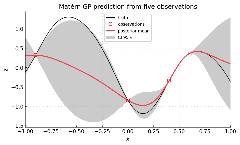
One-dimensional part: posterior means and variances on a regular grid. Red points are observations, the red curve is the posterior mean, and the shaded band is a pointwise 95 percent interval. The interval widens between observations and narrows at observed input locations. The full script also displays leave-one-out errors and truth-versus-prediction plots for the two-output case.

Source excerpt

# -----------------------------------
# Example 1: Single-output 1d problem
# -----------------------------------


# Define the problem
problem = gpc.ComputerExperiment(
    1,  # Input dimension
    [[-1], [1]],  # Input domain (box)
    single_function=gp.misc.testfunctions.twobumps,  # Test function
)

# Generate dataset
nt = 2000
xt = gp.misc.designs.regulargrid(problem.input_dim, nt, problem.input_box)
zt = problem(xt)

ind = [100, 1000, 1400, 1500, 1600]
ni = len(ind)
xi = xt[ind]
zi = problem(xi)

# Define the model, make predictions and draw conditional sample paths
model_choice = 1

if model_choice == 1:
    model = gpc.Model_ConstantMean_Maternp_REML(
        "1d_noisefree",
        problem.output_dim,
        mean_specification={"type": "constant"},
        covariance_specification={"p": 4},
    )
elif model_choice == 2:
    model = gpc.Model_ConstantMean_Maternp_REMAP(
        "1d_noisefree",
        problem.output_dim,
        mean_specification={"type": "constant"},
        covariance_specification={"p": 4},
    )
elif model_choice == 3:
    model = gpc.Model_ConstantMean_Maternp_ML(
        "1d_noisefree", problem.output_dim, covariance_specification={"p": 4}
    )

model.select_params(xi, zi)
model.run_diagnosis(xi, zi)
zpm, zpv = model.predict(xi, zi, xt)