Example 41: set inversion with BSS-style particles

Script: examples/example41_setinversion_smc.py

Purpose

The script estimates an inverse image with SetInversionBSS. It replaces the fixed grid of example40 by a particle population and moves from an initial box to a target box through an interpolation parameter mu. The particle update follows the BSS idea of representing a sequence of probability targets [1]. The box probabilities are the same type of Gaussian probabilities used in constrained Bayesian optimization [3].

What is computed

• posterior mean and variance at particle positions.

• the intermediate box B(mu) = (1 - mu) B_init + mu B_target.

• a target log-density proportional to box-membership probability inside the input box.

• SMC reweighting, resampling, and Markov moves of the particle population.

• box-membership probabilities and box weighted-MSE values at the current box.

Main objects

• gpmpcontrib.optim.setinversion.SetInversionBSS

• gpmpcontrib.SequentialStrategyBSS

• gpmp.mcmc.smc.SMC

Outputs

Run python examples/example41_setinversion_smc.py from the repository root to execute the example. Regenerate the static figure with cd docs && python make_example_results.py.

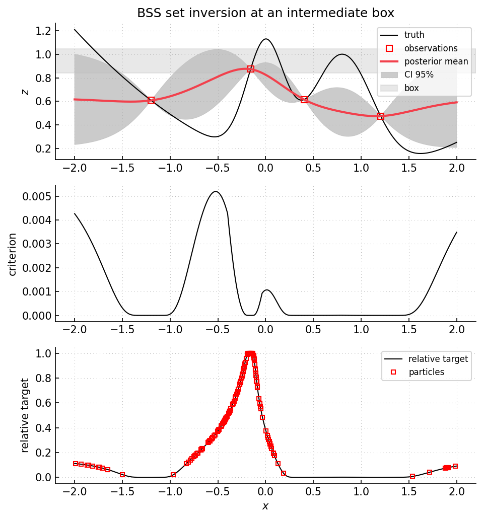
Intermediate output box with mu = 0.85. Lower panel: box-membership probability with SMC particles. Particle heights show the current target density up to a multiplicative constant.

Source excerpt

# -- define a mono-objective problem


problem = gpc.ComputerExperiment(
    1,  # dim of search space
    [[-2.0], [2.0]],  # search box
    single_function=test_function,  # test function
)


# -- create initial dataset

nt = 20 * 100
xt = gp.misc.designs.regulargrid(problem.input_dim, nt, problem.input_box)
zt = problem(xt)

ni = 4
ind = [i * 20 for i in [20, 46, 60, 80]]
xi = xt[ind]

# -- initialize a model and the ei algorithm

model = gpc.Model_ConstantMean_Maternp_REML(
    "GP1d",
    output_dim=problem.output_dim,
    mean_specification={"type": "constant"},
    covariance_specification={"p": 2},
)

box_init = gnp.array([[-0.0], [1.2]])
box_target = gnp.array([[0.99], [1.02]])

beta = 1.0
algo = si.SetInversionBSS(problem, model, box_init, box_target, options={"beta": beta})

algo.set_initial_design(xi)


# -- visualization


def plot(show=True, x=None, z=None):
    zpm, zpv = algo.predict(xt, convert_out=False)
    crit, _ = sampcrit.box_wMSE(algo.box_current, zpm, zpv)
    pe, _ = sampcrit.box_probability(algo.box_current, zpm, zpv)

    fig = gp.plot.Figure(nrows=3, ncols=1, isinteractive=True, figsize=(10, 8))
    fig.subplot(1)